Kansas Geological Survey, Open-file Report 2006-24
by
Julian Ivanov and Richard D. Miller
KGS Open-file Report 2006-24
for
Rob Huggins
Geometrics, Inc.
2190 Fortune Drive
San Jose, CA 95131
June 2006
The complete text of this report is available as an Adobe Acrobat PDF file.
Read the PDF version (516 kB)
The decomposition method is a reliable processing approach that provides clear, impulsive first-arrivals with sufficient bandwidth for consistent first-arrival energy picks from coded impulsive sequence data necessary for classic refraction or tomography analysis.
We worked on a 52-channel, 64000-sample multi-impact (wacker) seismic record (number 74) in SEG-2 format, provided by Geometrics. To overcome the 2-byte integer header limitation of the KGS header format, only every other input sample was used. As a result, output data had 32000 samples at 1-ms sampling interval. The impact sequence was recorded on the first trace (channel #24) as non-zero amplitude spikes with a cycle time of around 100 ms and zeros for the rest. During the conversion, amplitudes that were at half-ms times on channel 24 were lost. Thus, information for some of the impacts was lost. To overcome this problem we converted to KGS format (from multi-impact shot record 74) only the first 32766 samples at 0.5-ms sample interval. The resulting trace was 16383 ms long. Thus, all the impact sequence information for the first 32766 samples was accurately retrieved. Then the times were rounded to the nearest millisecond. In such a manner, a 1-ms sampling interval impact sequence was obtained. Amplitudes on all traces were normalized with respect to the largest amplitude in the impulse sequence. Relative impulse times and amplitudes from 155 impacts were retrieved (Table 1, at end of report) and available to decompose the multi-impact record. Forty-eight channels of record 74 were used for the tests discussed here.
A single-impact shot record (Figure 1a) is compared with the proposed decomposition method of a multi-impact shot record (Figure 1b), which is then compared to the traditional cross-correlation algorithm (Figure 1c). The first-arrivals on the decomposed shot (Figure 1b) match very well the first-arrivals of the single shot record (Figure 1a) and are also better defined than those on the cross-correlated shot (Figure 1c). In addition, the reflections on the decomposed shot (Figure 1b) seem to posses greatest S/N ratio and fidelity compared to the other two records.
Figure 1. a) Regular seismic single-impact shot record 59, b) multi-impact shot record 74 after decomposition using 155 impulses, c) multi-impact shot record 74 after cross-correlation using 155 impulses.
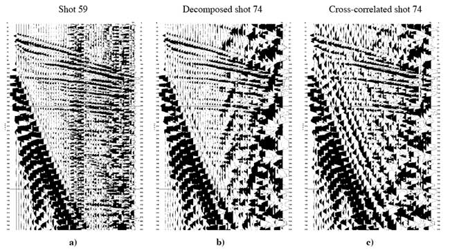
Figure 2. Low-cut filter 20-40 Hz applied to a) regular seismic single-impact shot record 59, b) multi-impact shot record 74 after decomposition using 155 impulses, c) multi-impact shot record 74 after cross-correlation using 155 impulses.
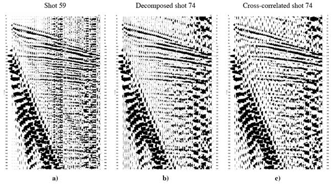
Figure 3. Low-cut filter 30-60 Hz applied to a) regular seismic single-impact shot record 59, b) multi-impact shot record 74 after decomposition using 155 impulses, c) multi-impact shot record 74 after cross-correlation using 155 impulses.
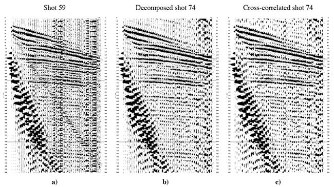
Again, the decomposed shot gather (Figure 3b) seems to have better coherency and signal-to-noise ratio first-arrivals and reflections. Optimizing the low-cut filter also seemed to enhance the first-arrival energy of the cross-correlated shot record (Figure 3c); however, this enhancement comes at a price, first-arrival-wavelet phase distortion. Such phase distortion can be an obstacle for some analysis techniques.
In this instance, filtering seemed to have removed the low-frequency component of the surface-wave, which probably stacked in during the cross-correlation process (because during the impact sequence generation surface-wave from a previous impact affects the record) and hence its appearance prior to the first-arrivals. In most cases successful surface-wave filtering is challenging and generally results in phase distortion of the first-arrival wavelet, making it difficult to recognize the actual onset of first-arrival energy.
We selected data from channel 27 (third trace from the left on shot records) to compare wavelets from the different data sets. Channel 27 was extracted from the single-impact shot record 59 (Figure 1a), from the decomposed shot 74 (Figure 1b), from the cross-correlated shot 74 (Figure 1c), from the 30-60-Hz low-cut filtered decomposed shot 74 (Figure 3b), and from the 30-60-Hz low-cut filtered cross-correlated shot 74 (Figure 3c). All the traces were gathered into a single trace gather No 5974 and their channel numbers were renumbered (Figure 4).
Figure 4. The first 100 ms of 1000 ms are displayed to better observe the first-arrival wavelet. A common trace gather is displayed using identical channel numbers from five different shot gathers. The first trace is from the single-impact shot record 59, the second trace is from the decomposed shot 74, the third trace is from the cross-correlated shot 74, the forth trace is from the 30-60-Hz low-cut filtered decomposed shot 74, and the fifth trace is from the 30-60-Hz low-cut filtered cross-correlated shot 74.
To numerically evaluate the match between the traces, the first trace was cross-correlated with all the traces. The corresponding cross-correlation coefficients between trace 1 and the rest of traces from the common trace gather are as follows:
| Trace number | Coefficient |
|---|---|
| 1 | 1.000000 |
| 2 | 0.940079 |
| 3 | 0.884428 |
| 4 | 0.681591 |
| 5 | 0.660563 |
It is evident from the above data that trace 1, from the single-impact shot record 59, correlates best with trace 2, which is from the decomposed shot 74.
Comparing the frequency spectra of the five traces (Figure 5) provides additional information about the data. The trace from the single-impact shot record 59 has better frequency content than the trace from the decomposed shot 74 (Figure 5). At the present moment any degradation in spectra due to the decomposing algorithm is not expected. Therefore, the richer frequency content of trace number 1 could be because the single-shot record contains more high-frequency noise (i.e. air wave, ambient noise, etc.) than the decomposed record. However, the trace from the decomposed shot has the richest frequency content compared to the rest of the traces.
Figure 5. Frequency spectra of the five traces from the combined shot gather 5974. The red line with triangles is from the single-impact shot record 59, the green line with circles is from the decomposed shot 74, the light blue line with squares is from the cross-correlated shot 74, the black line is from the 30-60-Hz low-cut filtered decomposed shot 74, and the blue line with stars is from the 30-60-Hz low-cut filtered cross-correlated shot 74.
The first 70 ms of all the traces were graphically displayed for closer observation (Figure 6). It is evident that the decomposed trace has greatest similarity with the single-impact trace. The 1-ms shift of the decomposed trace, necessary to make the match, is likely related to different near-surface conditions, which affected the travel-time and frequency content of the wacker and single-impact data differently.
Figure 6. First-arrival wavelet comparison of channel 57 from the corresponding record. The decomposed trace was shifted (delayed) with 1 ms for better match with the single-impact shot.
We used a first-arrival automatic picker (developed at the KGS) to determine which data set was best suited to automatic routines for first-arrival picking. The software requires manual selection of an initial starting point and a range of traces to estimate the first-arrivals. Accordingly, we selected the starting point for first-arrival picking to be channel 26 (trace #2) at 20 ms and the range of traces from channel 26 to channel 65 (trace #41). The first-arrival picker estimated the first-arrivals for channels 26 through 45 well and failed for channels 46 to 65 because of the noise, specifically noise on channels 48 to 52 (Figure 7).
Figure 7. First-arrival picking on the single-impact shot record 59.
Using the same starting point and range of traces, the first-arrival picker had fewer difficulties on the decomposed record. The first-arrivals for channels 26 through 58 were estimated fairly well, but the picker failed for channels 59 to 65 because of the noise (Figure 8).
Figure 8. First-arrival picking on the decomposed shot 74.
The first-arrival picker performed poorly (using the same parameters) on the cross-correlated record. It was misguided by low-frequency noise on channels 31 through 40 and failed because of the noise on channels 59 to 65 (Figure 9).
Figure 9. First-arrival picking on the cross-correlated shot 74.
The first-arrival picker performed best on the low-cut filtered shots, both decomposed (Figure 10) and cross-correlated (Figure 11); picking quality was nearly identical. Low-cut filters usually cause phase-shift (time shift) errors, a problem evident on these data. Considering the possibility of phase shift errors due to low-cut filtering, the decomposed shot gather appears to be the best candidate for first-arrival picking.
Figure 10. First-arrival picking on the 30-60-Hz low-cut filtered decomposed shot 74.
Figure 11. First-arrival picking on the 30-60-Hz low-cut filtered cross-correlated shot 74.
Random or precise-interval impact sequences are not necessary for the decomposition method. Randomness is not a requirement. At the present moment, knowing the time and the amplitude of the impact sequence are the only requirements for decomposing the multi-impact data. This could be tested if non-random data are provided.
Further test with this data showed that decomposing data with a number of impacts lesser than 155 may still provide good enough quality for the purposes of first-arrival picking.
The decomposed data have better frequency content than the cross-correlated data (Figure 5), its first-arrival shape matches best and is almost identical to the first-arrival pattern on the single-impact shot, and it is most accurate for first-arrival picking by the automatic picker used.
Furthermore, when examining the reflection events at 190 ms, 250 ms, and 300 ms (Figures 1, 2, and 3), the decomposed data provide more continuous reflections with higher signal-to-noise ratio then the other data sets.
Table 1. Impact sequence of 155 impulses.
| TraceTime | Value |
|---|---|
| 50 | 0.4273 |
| 150 | 0.395 |
| 243 | 0.3641 |
| 329 | 0.4466 |
| 418 | 0.4336 |
| 512 | 0.4425 |
| 615 | 0.4256 |
| 713 | 0.4064 |
| 953 | 0.1775 |
| 1083 | 0.7178 |
| 1187 | 0.5482 |
| 1295 | 0.1364 |
| 1375 | 0.2807 |
| 1469 | 0.2354 |
| 1556 | 0.3669 |
| 1644 | 0.2699 |
| 1728 | 0.465 |
| 1823 | 0.3791 |
| 1921 | 0.4089 |
| 2020 | 0.5139 |
| 2116 | 0.4033 |
| 2205 | 0.2776 |
| 2300 | 0.2794 |
| 2399 | 0.4402 |
| 2520 | 0.4409 |
| 2619 | 0.3023 |
| 2706 | 0.4214 |
| 2796 | 0.4636 |
| 2882 | 0.5474 |
| 2969 | 0.5174 |
| 3059 | 0.5445 |
| 3153 | 0.4679 |
| 3244 | 0.8082 |
| 3331 | 0.7231 |
| 3428 | 0.433 |
| 3527 | 0.46 |
| 3633 | 0.3399 |
| 3846 | 0.1242 |
| 4161 | 0.5634 |
| 4267 | 0.6888 |
| 4376 | 0.5988 |
| 4475 | 0.2327 |
| 4557 | 0.4306 |
| 4657 | 0.4229 |
| 4757 | 0.3562 |
| 4857 | 0.4228 |
| 4991 | 0.1271 |
| 5075 | 0.3973 |
| 5174 | 0.6907 |
| 5260 | 0.5411 |
| 5353 | 0.447 |
| 5439 | 0.5208 |
| 5527 | 0.4846 |
| 5611 | 0.5193 |
| 5709 | 0.4785 |
| 5810 | 0.2445 |
| 5914 | 0.6072 |
| 6023 | 0.3711 |
| 6217 | 0.6607 |
| 6357 | 0.2813 |
| 6450 | 0.4416 |
| 6539 | 0.6599 |
| 6631 | 0.6098 |
| 6716 | 0.614 |
| 6804 | 0.5186 |
| 6889 | 0.5974 |
| 6984 | 0.449 |
| 7071 | 0.7703 |
| 7168 | 0.4102 |
| 7251 | 0.611 |
| 7351 | 0.5138 |
| 7447 | 0.4844 |
| 7566 | 0.5865 |
| 7725 | 0.0619 |
| 7816 | 0.1588 |
| 8095 | 0.7068 |
| 8187 | 0.6875 |
| 8280 | 0.5752 |
| 8368 | 0.3511 |
| 8449 | 0.6308 |
| 8538 | 0.7221 |
| 8621 | 0.7034 |
| 8709 | 0.593 |
| 8792 | 0.581 |
| 8882 | 0.4625 |
| 8961 | 0.6085 |
| 9057 | 0.4251 |
| 9136 | 0.7232 |
| 9238 | 0.3107 |
| 9322 | 0.6669 |
| 9439 | 0.5051 |
| 9546 | 0.3787 |
| 9687 | 0.472 |
| 9796 | 0.6209 |
| 9891 | 0.8673 |
| 10001 | 0.4824 |
| 10125 | 0.2735 |
| 10226 | 0.2496 |
| 10359 | 0.1242 |
| 10442 | 0.4586 |
| 10549 | 0.7873 |
| 10641 | 0.6636 |
| 10741 | 0.4768 |
| 10844 | 0.0613 |
| 10917 | 0.589 |
| 11022 | 0.4124 |
| 11123 | 0.6111 |
| 11221 | 0.2354 |
| 11296 | 1 |
| 11392 | 0.6714 |
| 11482 | 0.5736 |
| 11571 | 0.2624 |
| 11648 | 0.617 |
| 11753 | 0.3828 |
| 11843 | 0.6102 |
| 11937 | 0.4991 |
| 12024 | 0.3648 |
| 12107 | 0.5039 |
| 12196 | 0.6108 |
| 12294 | 0.6319 |
| 12395 | 0.6923 |
| 12490 | 0.7483 |
| 12593 | 0.6034 |
| 12761 | 0.8781 |
| 12862 | 0.819 |
| 12953 | 0.4677 |
| 13052 | 0.4999 |
| 13153 | 0.5933 |
| 13291 | 0.6912 |
| 13684 | 0.1748 |
| 13995 | 0.8377 |
| 14104 | 0.781 |
| 14210 | 0.7144 |
| 14313 | 0.4133 |
| 14394 | 0.7002 |
| 14489 | 0.6815 |
| 14571 | 0.631 |
| 14663 | 0.4711 |
| 14748 | 0.6656 |
| 14844 | 0.5638 |
| 14930 | 0.6745 |
| 15027 | 0.4924 |
| 15112 | 0.7296 |
| 15218 | 0.4851 |
| 15311 | 0.5395 |
| 15415 | 0.5586 |
| 15514 | 0.4809 |
| 15615 | 0.4404 |
| 15716 | 0.2653 |
| 15821 | 0.3895 |
| 15934 | 0.5447 |
| 16041 | 0.5764 |
| 16147 | 0.6174 |
| 16253 | 0.3629 |
| 16353 | 0.2781 |
Kansas Geological Survey, Geophysics
Placed online July 12, 2006
Comments to webadmin@kgs.ku.edu
The URL for this page is http://www.kgs.ku.edu/Geophysics/OFR/2006/OFR06_24/index.html