Kansas Geological Survey, Open-file Report 2006-1
by
Jianghai Xia
KGS Open-file Report 2006-1
for
Andrew Weinberg
Bechtel-S Corp.
203 E. Milton St.
Austin, TX 78704
June 2006
A recently developed technique--Multichannel Analysis of Surface Waves (MASW, Park et al., 1999, Xia et al., 1999)--was used to detect shallow geological features (< 150 ft) at Maxwell AFB in Montgomery, Alabama. The MASW method with the standard common depth point (CDP) roll-along acquisition format (Mayne, 1962) was employed to acquire surface-wave data along eight lines with a total length of 7,712 ft. S-wave velocity and residual velocity sections were generated. Notable changes in shear (S)-wave velocities reveal a possible buried channel and interfaces between different rocks. S-wave velocities inverted from the MASW method normally possess 10-15% error compared to direct borehole measurements (Xia et al., 2002a). In addition, the vertical and horizontal resolution of the results is limited by the geophone spread and the layered earth model used in the inversion. Therefore, anyone who interprets the S-wave velocity and residual velocity sections should be aware of the uncertainty and these limitations.
Surface waves are guided and dispersive. In the case of one layer on top of a solid homogenous half-space, dispersion of the Rayleigh wave occurs when the wavelengths of the Rayleigh wave are in the range of 1 to 30 times the layer thickness (Stokoe et al., 1994). Longer wavelengths penetrate deeper than shorter wavelengths for a given mode, generally exhibit greater phase velocities, and are more sensitive to the elastic properties of the deeper layers (p. 30, Babuska and Cara, 1991). Shorter wavelengths are sensitive to the physical properties of surficial layers. For this reason, a particular mode of surface wave will possess a unique phase velocity for each unique wavelength, thus, leading to the dispersion of the seismic signal.
Shallow (< 150 ft) geological features can be difficult to detect from surface investigations and many times provide an expensive challenge to detection with hit and miss drilling. Stokoe and Nazarian (1983) and Nazarian et al. (1983) present a surface-wave method, called Spectral Analysis of Surface Waves (SASW), that analyzes the dispersion curve of ground roll to produce near-surface S-wave velocity profiles to image targets significant to shallow engineering, environmental, and groundwater studies.
A recently developed technique--Multichannel Analysis of Surface Waves (MASW)--provides a feasible tool to detect shallow geological features (Park et al., 1999, Xia et al., 1999). With utilization of a multichannel system, data acquisition is more efficient, noise recognition and suppression are easier and more effective, and determination of dispersion curves is more accurate. Based on their experience (e.g., Xia et al., 2002a), the fundamental-mode phase velocities can generally provide reliable S-wave velocities (±15%). The accuracy can be increased if higher modes of surface waves are available and included in the inversion process (Xia et al., 2002a and 2003). Recent advances in the use of surface waves for near-surface imaging incorporated the MASW method (Park et al., 1996, and 1999; Xia et al., 1997, 1998, 1999, 2002b, 2004a, and 2005) with a standard common depth point (CDP) roll-along acquisition format (Mayne, 1962) similar to conventional petroleum exploration data acquisition. Combining these two uniquely different approaches to acoustic imaging of the subsurface allows high confidence, non-invasive delineation of horizontal and vertical variations in near-surface material properties (Miller et al., 1999, Xia et al., 1998). Practical guidelines for surface-wave data acquisition and processing (Xia et al., in press (a)) and utilizing surface-wave in a nonlayered earth model were discussed (Xia et al., in press (b)). Feasibility of directly detecting voids with Rayleigh-wave diffraction was studied (Xia et al., in review).
Notable changes in S-wave velocity are expected at boundaries between different materials. The goal of this project is to map a buried channel or anomalous zones at Maxwell AFB in Montgomery, Alabama. The target depth is 30-100 ft below surface level (bsl) but images are desired to 150 ft bsl. Locating these areas allows remediation before they become a hazard to human health or the environment. Surface-wave data were collected along eight lines with a total length of 7,712 ft. S-wave velocity sections were generated These sections delineate several velocity-low spots that are interpreted as a possible buried channel and velocity interfaces that could reveal changes of rock types. Due to the limited horizontal resolution of the imaging method and accuracy of the MASW method, features interpreted in S-wave velocity sections may not directly reflect subsurface geology.
Surface-wave imaging has shown great promise in detecting shallow tunnels (Xia et al., 1998) and bedrock surfaces (Miller et al., 1999). Extending this imaging technology to include lateral variations in lithology has required a unique approach incorporating MASW and CDP methods. Integrating these techniques provides a 2-D continuous shear-wave velocity profile of the subsurface. Signal enhancement resulting from determination of a dispersion curve using upwards of 48 or so closely spaced receiving channels and the calculation of a dispersion curve every 2-8 ft along the ground surface provides a unique, relatively continuous view of the shallow subsurface. This highly redundant method enhances the accuracy of the calculated shear wave velocity and minimizes the likelihood that the irregularities associated with an occasional erratic dispersion curve will corrupt the data analysis.
The MASW method is based on the fact that the S-wave velocity is the dominant influence on Rayleigh wave for a layered earth model, which assures us that inverting phase velocities will give us an S-wave velocity profile (1-D S-wave velocity function, Vs vs. depth) at the center of a geophone spread. Because data are acquired in the standard CDP format, phase velocities of ground roll can be extracted from each shot gather so that numerous 1-D S-wave profiles along a survey line can be generated. A two-dimensional (2-D) vertical S-wave velocity section can be generated by any contouring software.
A number of multichannel records should first be collected in the standard CDP roll-along acquisition format. If a swept source is used, the recorded data should be converted into a correlated format (Mayne, 1962), which is equivalent to data acquired with an impulsive source. Surface impact sources and receivers with a low-response frequency, normally less than 8 Hz, are commonly chosen to acquire surface-wave data. Data-acquisition parameters, such as source-receiver offset, receiver spacing, geophone spread, etc., should be set to enhance ground-roll signals (Xia et al., 2004b and in press (a)).
Once the data collection is completed, phase velocities (dispersion curves) of the ground roll of each shot gather should be calculated. The frequency range and phase-velocity range of the ground roll need to be determined by analyzing data along the entire line. These two ranges are very important constraints to correctly extract the dispersion curve from each shot gather. They not only help eliminate noise such as body wave, higher mode of Rayleigh waves, etc., during calculation of phase velocities (Park et al., 1999), but they also assist in defining the thickness of the layer model.
Inversion should be performed on each dispersion curve to generate an S-wave velocity vs. depth profile (Xia et al., 1999). The inverted S-wave velocity profile should be located in the middle of the receiver spread (Miller and Xia, 1999). Initial models are a key factor to assure convergence of the inversion process. After processing more than five thousand shots of real data and countless sets of modeling data, initial models defined by Xia et al.'s algorithm (1999) are generally converged to models that are acceptable in geology and also fit the dispersion curve in a given error range. The number of layers is chosen between five and twenty in our experience, based on the accuracy of surface-wave data, the investigation depth, and required resolution of S-wave velocity. The thickness of each layer varies based on the depth(s) of interest. For example, for a geological problem with a depth of interest of 50-100 ft we may choose a 10-layer model with the first three layers being 3 ft thick, the next three layers 6 ft thick, the last three layers 10 ft thick, and a half space. The inverted S-wave velocity profile for each shot gather is the result of horizontally averaging across the length of the geophone spread.
Gridding algorithms, such as kriging, minimum curvature, etc., may be used to generate a 2-D contour map of the S-wave velocity of a vertical section. With density information, a shear modulus section can be generated simultaneously. Two-dimensional data processing techniques, such as regression analysis, can be easily applied to a vertical section of S-wave velocity to enhance local anomalies.
The general procedure for generating a 2-D S-wave velocity map is summarized as follows (Figure 1):
Figure 1. A diagram of construction of 2-D S-wave velocity map by the MASW method. Rayleigh-wave phase velocities are extracted from the field data in the F-K domain. Phase velocities are inverted for a shear-wave velocity profile (Vs vs. depth). After a number of S-wave velocity profiles are generated when a seismic source is moving along a line, finally, a 2-D S-wave velocity map is generated with contouring software.
On a 2-D S-wave velocity map, the bedrock surface is usually associated with high S-wave velocity gradients, while fracture zones, voids, buried landfill edges, and the like may be indicated by S-wave anomalies such as low-velocity zones.
The maximum investigation depth of the project was around 150 ft. As rule of thumb, the nearest offset (A in Figure 2) is approximately equal to the maximum investigation depth (Xia et al., 2004b). Because 48-channel system was available, I decided to set the nearest offset to 40 ft to ensure high-frequency signals were recorded. The geophone interval (B in Figure 2) was set to 8 ft. With the 48-channel system, the geophone spread (C in Figure 2) is 376 ft, which implies that in the best scenario the longest recorded wavelength could be 376 ft. The maximum investigation depth is normally half of the longest wavelength (Rix and Leipski, 1991). With this field setting, the maximum investigation depth could reach 180 ft bsl. In reality, the recorded longest wavelength is usually shorter than the geophone spread due to band-limited source and geophone, ambient noise, energy attenuation, and complexity of near-surface geology.
Figure 2. Three field-data-acquisition parameters: A. The nearest source-receiver offset: approximately equal to the maximum investigation depth; B. Receiver spacing: the thinnest layer of the layer model; and C. Receiver spread--distance between the first receiver and the last receiver: approx. 2 times the maximum investigation depth.
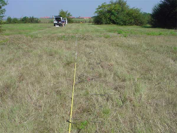
Multichannel records were acquired using the end-on geophone spread with Geometrics Geodes (Figure 3a) and forty-eight 4.5-Hz vertical-component geophones (Figure 3b). The source was a 12-lb hammer (Figure 3c) vertically impacting a 1 ft by 1 ft metal plate. Data were recorded on a notebook directly (Figure 3d). Recording time was 2 s with a 1-ms sample interval. No acquisition filter was applied during the recording. To increase signal to noise (S/N) ratio, two blows at each station were vertically stacked.
Figure 3a. One of four Geodes used in data acquisition.
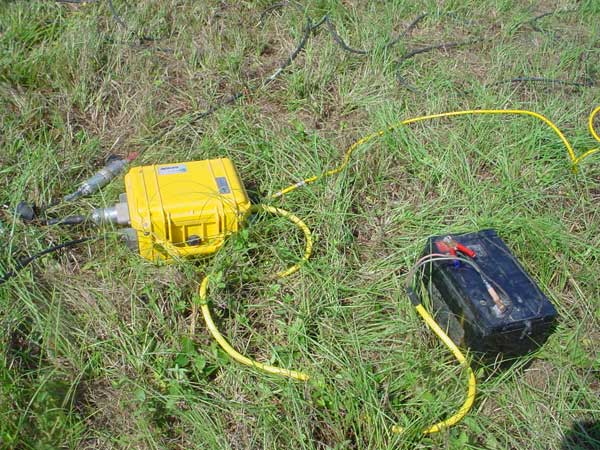
Figure 3b. A 4.5-Hz vertical component geophone.
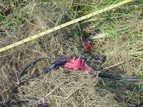
Figure 3c. A 12-lb hammer vertically impacts a 1 ft by 1 ft metal plate as a seismic source. Karlin Yudichak of Geophex Ltd. was swinging the hammer.
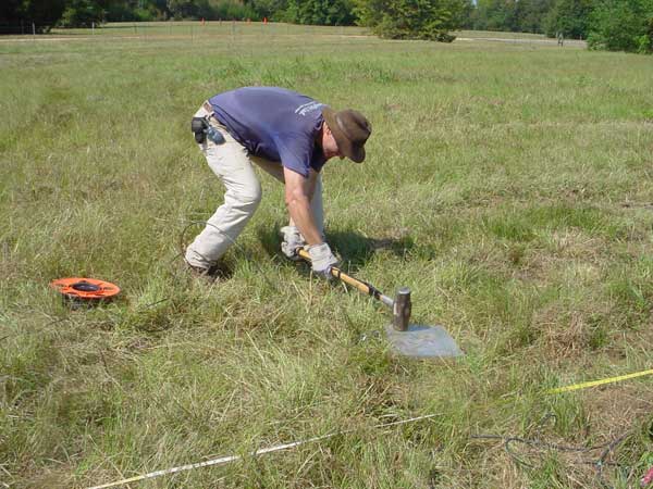
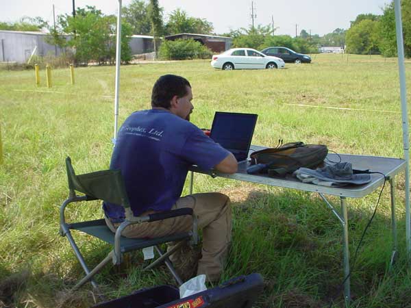
Figure 3d. A notebook was used to record data. Brad Carr of Geophex Ltd. was assessing data.
A seismic crew from Geophex Ltd. performed data acquisition. Surface-wave data were collected along eight lines. The total length of the eight lines is 7,712 ft with an imaging length of 6,416 ft (Figure 4).
Figure 4. Surface-wave data were acquired along eight lines. Geographic locations of the lines can be determined by the locations of the wells.
Limited and uniform preprocessing was applied to the data to minimize processing artifacts.
Figures 5-12 show data examples from each line. F-K filtered data (Figures 5b-10b) show the success of removing weak back scattering (Figures 5a-7a) and relatively strong back scattering (Figures 8a-10a). F-K filtered data (Figures 11b-12b) show that the F-K filter did not damage data when there was no significant back scattering (Figures 11a-12a).
Figure 5. An example from line 1. a) Raw data.
Figure 5. An example from line 1. b) F-K filtered data.
Figure 5. An example from line 1. c) Dispersion curve in the f-v domain.
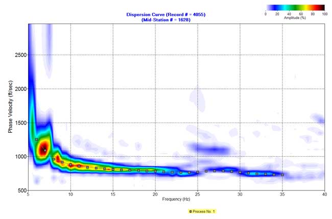
Figure 5. An example from line 1. d) Inverted S-wave velocity.
Figure 6. An example from line 2. a) Raw data.
Figure 6. An example from line 2. b) F-K filtered data.
Figure 6. An example from line 2. c) Dispersion curve in the f-v domain.
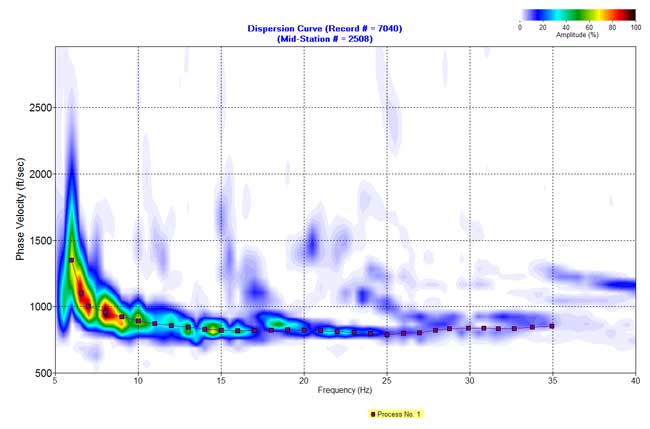
Figure 6. An example from line 2. d) Inverted S-wave velocity.
Figure 7. An example from line 3. a) Raw data.
Figure 7. An example from line 3. b) F-K filtered data.
Figure 7. An example from line 3. c) Dispersion curve in the f-v domain.
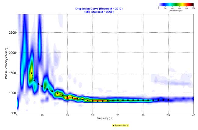
Figure 7. An example from line 3. d) Inverted S-wave velocity.
Figure 8. An example from line 4. a) Raw data.
Figure 8. An example from line 4. b) F-K filtered data.
Figure 8. An example from line 4. c) Dispersion curve in the f-v domain.
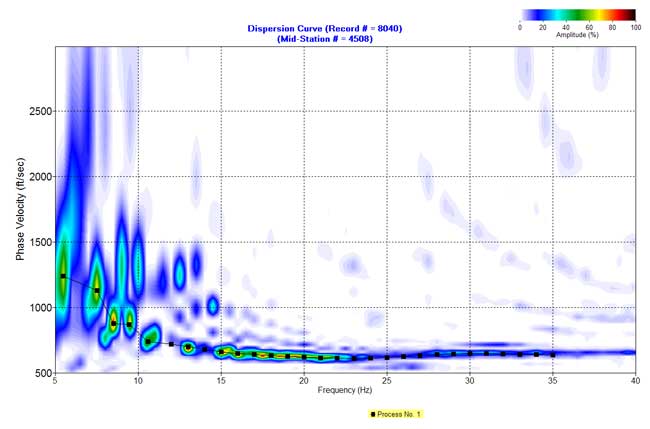
Figure 8. An example from line 4. d) Inverted S-wave velocity.
Figure 9. An example from line 5. a) Raw data.
Figure 9. An example from line 5. b) F-K filtered data.
Figure 9. An example from line 5. c) Dispersion curve in the f-v domain.
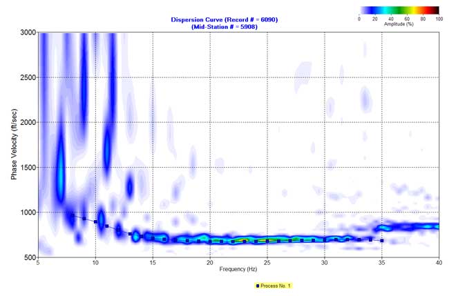
Figure 9. An example from line 5. d) Inverted S-wave velocity.
Figure 10. An example from line 6. a) Raw data.
Figure 10. An example from line 6. b) F-K filtered data.
Figure 10. An example from line 5. c) Dispersion curve in the f-v domain.
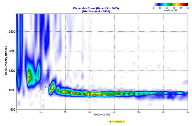
Figure 10. An example from line 5. d) Inverted S-wave velocity.
Figure 11. An example from line 7. a) Raw data.
Figure 11. An example from line 7. b) F-K filtered data.
Figure 11. An example from line 7. c) Dispersion curve in the f-v domain.
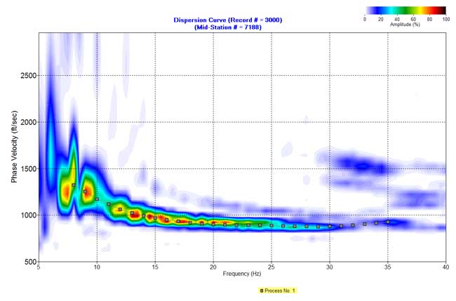
Figure 11. An example from line 7. d) Inverted S-wave velocity.
Figure 12. An example from line 8. a) Raw data.
Figure 12. An example from line 8. b) F-K filtered data.
Figure 12. An example from line 8. c) Dispersion curve in the f-v domain.
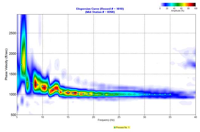
Figure 12. An example from line 8. d) Inverted S-wave velocity.
F-K filtered data (Figures 5b-12b) were used to produce dispersion-curve images in the frequency-velocity (f-v) domain (Figure 5c-12c). These examples show the wavelength of surface waves in the range of 15-170 ft is from 7 to 35 Hz. I manually picked phase velocities (dispersion curve) from each dispersion image to ensure the right velocity selection at each frequency.
Inversion was performed on these dispersion curves to generate an S-wave velocity profile (Figures 5d-12d) placed at the center of the geophone spread. A 2-D contour map of the S-wave velocity for each line (Figures 13a-20a) and residual S-wave velocity sections (Figures 13b-20b) that were obtained by removing the second-order trend of S-wave velocity to enhance local anomalies were generated by SurferTM.
Figure 13a. S-wave velocity section of line 1.
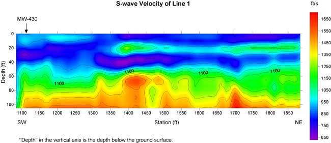
Figure 13b. Residual S-wave velocity section of line 1 with a second-order trend removed from Figure 13a.
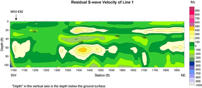
Figure 14a. S-wave velocity section of line 2.
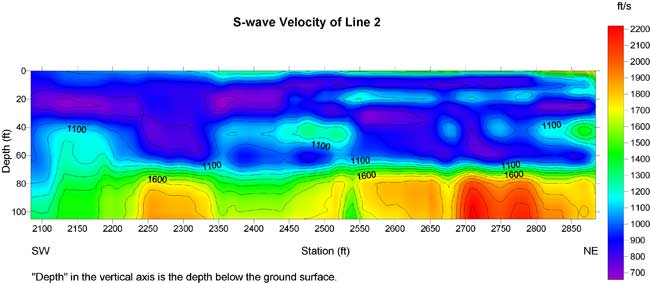
Figure 14b. Residual S-wave velocity section of line 2 with a second-order trend removed from Figure 14a.
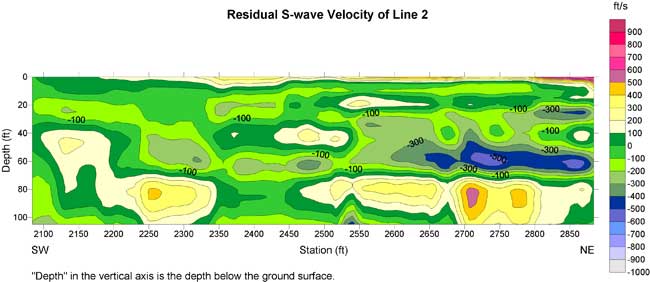
Figure 15a. S-wave velocity section of line 3. A thick contour line (1400 ft/s) may indicate a geological interface.
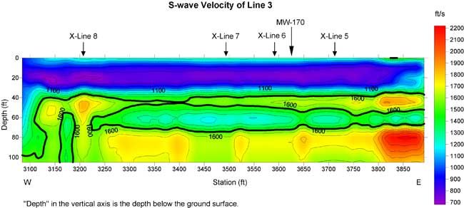
Figure 15b. Residual S-wave velocity section of line 3 with a second-order trend removed from Figure 15a.
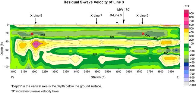
Figure 16a. S-wave velocity section of line 4. A thick contour line (1400 ft/s) may indicate a geological interface.
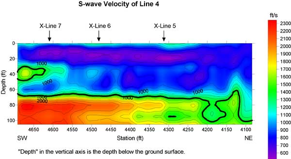
Figure 16b. Residual S-wave velocity section of line 4 with a second-order trend removed from Figure 16a.
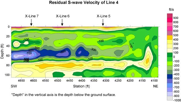
Figure 17a. S-wave velocity section of line 5. A thick contour line (1400 ft/s) may indicate a geological interface.
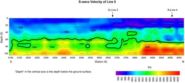
Figure 17b. Residual S-wave velocity section of line 5 with a second-order trend removed from Figure 17a.
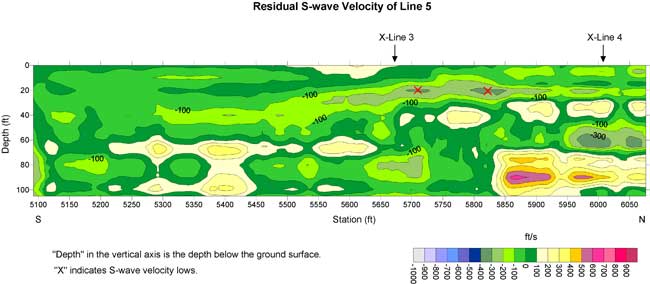
Figure 18a. S-wave velocity section of line 6. A thick contour line (1400 ft/s) may indicate a geological interface.
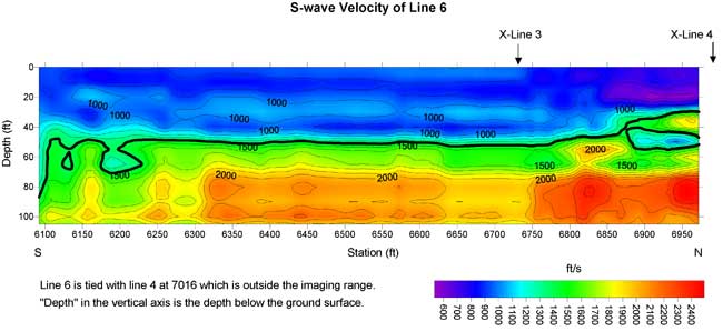
Figure 18b. Residual S-wave velocity section of line 6 with a second-order trend removed from Figure 18a.
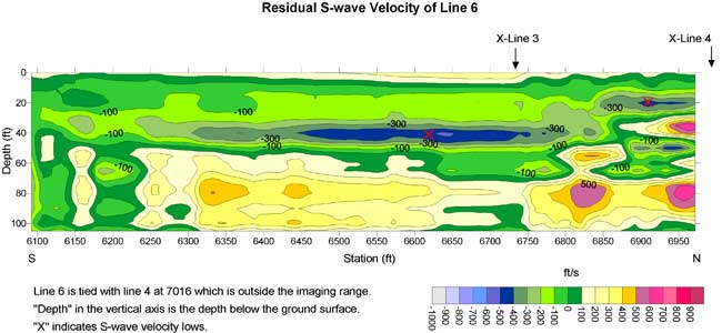
Figure 19a. S-wave velocity section of line 7. A thick contour line (1600 ft/s) may indicate a geological interface.
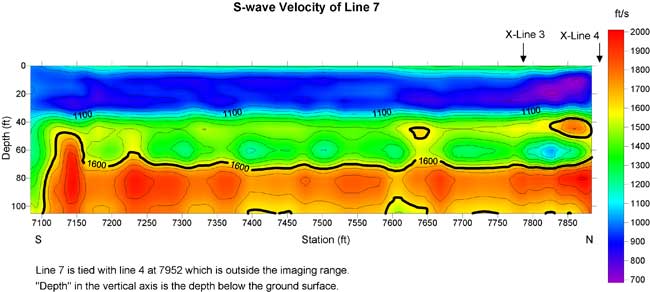
Figure 19b. Residual S-wave velocity section of line 7 with a second-order trend removed from Figure 19a.
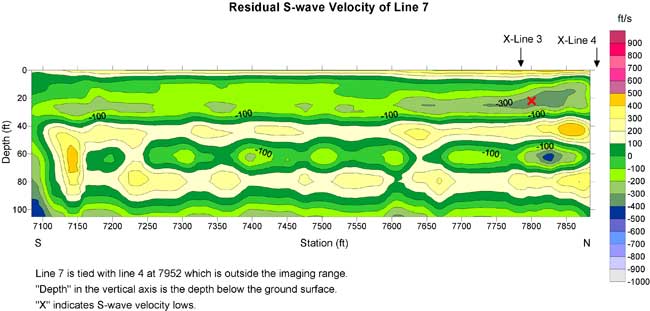
Figure 20a. S-wave velocity section of line 8. A thick contour line (1600 ft/s) may indicate a geological interface.
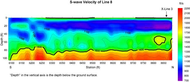
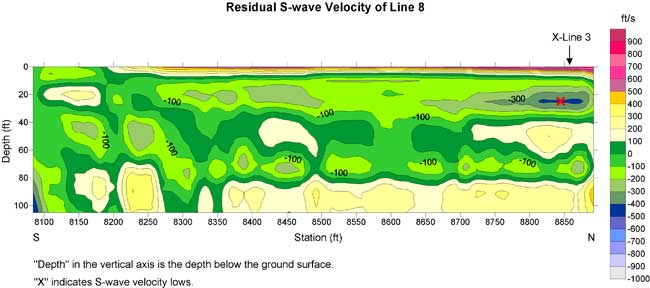
Figure 20b. Residual S-wave velocity section of line 8 with a second-order trend removed from Figure 19a.
Direct interpretations based on S-wave velocity sections and residual S-wave velocity sections would be possible in most cases. A minimum interpretation is given as follows.
A geological interface may be associated with a rapid change of velocity. I drew a thick contour line on Figures 15a-20a. The contour is in the range of 1400-1600 ft/s. The location of the contour line corresponds to the maximum gradient of S-wave velocity. This contour line is probably indicative of a geological interface.
Both the surficial aquifer and the Eutaw aquifer possess relatively high S-wave velocities shown in yellow to pink in residual S-wave velocity sections (Figures 13b-20b).
Normally a buried channel possesses a relatively low S-wave velocity in comparison to surrounding materials. I marked "X" on S-wave velocity lows in the residual S-wave velocity sections of line 3 and lines 5 to 8. The low around 5700 on line 5 could be due to the ditch. Lows with depths of 10 to 30 ft were used to construct a plan view of this interpreted buried channel. I did not use the low at the depth of 40 ft and centered at 6625 on line 6 in the construction of a possible buried channel (Figure 21). I believe this 300-ft-long velocity low may be caused by some other geological feature.
Figure 21. A plan view of a possible buried channel in blue interpreted from residual S-wave velocity sections. Depth of the channel is around 20 ft below the ground surface.
S-wave velocities inverted from the MASW method normally possess 10-15% error compared to direct borehole measurements (Xia et al., 2002a). In addition, the vertical and horizontal resolution of the results is limited by the geophone spread and the layered earth model used in the inversion. Therefore, velocity interfaces may not necessarily be geological interfaces.
Mismatches of S-wave velocities at intersections of line 3 with lines 5 to 8 are notable. This phenomenon is not uncommon with current surface-wave techniques. S-wave velocities inverted from data acquired along two lines in different directions are usually different not only due to 10-15% error in S-wave velocity determined by the MASW method but also to 1) anisotropy of the sediments, especially S-wave splitting in a polar anisotropic medium, and/or 2) S-wave velocities of different materials (layers are not horizontal within geophone spreads in two different directions).
S-wave velocities are about 1300 ft/s for clay and 1750 ft/s for saturated sand and gravel (McLamore et al., 1978). Because of the limitations of the MASW method and the relatively small difference between saturated sand/gravel and clay at this site, I am not surprised that surface-wave results did not reveal the regional dip to the south and west on the top of the clay surface.
The author thanks Marla Adkins-Heljeson and Mary Brohammer of the Kansas Geological Survey for editing the report.
Babuska, V., and Cara, M., 1991, Seismic anisotropy in the Earth: Kluwer Academic Publishers, Boston.
Mayne, W.H., 1962, Horizontal data stacking techniques: Supplement to Geophysics, 27, 927-938.
McLamore, V.R., Anderson, D.G., and Espana, C., 1978, Crosshole testing using explosive and mechanical energy sources; in, Dynamic Geotechnical Testing ASTM STP 654: ASTM, 30-50.
Miller, R.D., and Xia, J., 1999, Feasibility of seismic techniques to delineate dissolution features in the upper 600 ft at Alabama Electric Cooperative's proposed Damascus site, Interim Report: Kansas Geological Survey, Open-file Report 99-3.
Miller, R.D., Xia, J., Park, C.B., and Ivanov, J., 1999, Multichannel analysis of surface waves to map bedrock: The Leading Edge, 18, 1392-1396.
Nazarian, S., Stokoe II, K.H., and Hudson, W.R., 1983, Use of spectral analysis of surface waves method for determination of moduli and thicknesses of pavement systems: Transportation Research Record No. 930, 38-45.
Park, C.B., Miller, R.D., and Xia, J., 1996, Multi-channel analysis of surface waves using Vibroseis [Exp. Abs.]: Soc. of Expl. Geophys., 66th Annual Meeting, Denver, Colorado, 68-71.
Park, C.B., Miller, R.D., and Xia, J., 1999, Multi-channel analysis of surface waves: Geophysics, 64, 800-808.
Rix, G.J., and Leipski, E.A., 1991, Accuracy and resolution of surface wave inversion, in, Bhatia, S.K., and Blaney, G.W., Eds., Recent advances in instrumentation, data acquisition and testing in soil dynamics: Am. Soc. Civil Eng., 17-32.
Stokoe II, K.H., and Nazarian, S., 1983, Effectiveness of ground improvement from spectral analysis of surface waves: Proceeding of the Eighth European Conference on Soil Mechanics and Foundation Engineering, Helsinki, Finland.
Stokoe II, K.H., Wright, G.W., Bay, J.A., and Roesset, J.M., 1994, Characterization of geotechnical sites by SASW method, in, Geophysical characterization of sites, edited by R. D. Woods: ISSMFE Technical Committee #10, XIII ICSMFE, New Delhi, India, pp. 15-25.
Xia, J., Miller, R.D., and Park, C.B., 1997, Estimation of shear wave velocity in a compressible Gibson half-space by inverting Rayleigh wave phase velocity: Technical Program with Biographies, SEG, 67th Annual Meeting, Dallas, TX, 1927-1920.
Xia, J., Miller, R.D., and Park, C.B., 1998, Construction of vertical seismic section of near-surface shear-wave velocity from ground roll [Exp. Abs.]: Soc. Explor. Geophys./AEGE/CPS, Beijing, 29-33.
Xia, J., Miller, R.D., and Park, C.B., 1999, Estimation of near-surface shear-wave velocity by inversion of Rayleigh wave: Geophysics, 64, 691-700.
Xia, J., Miller, R.D., Park, C.B., Hunter, J.A., Harris, J.B., and Ivanov, J., 2002a, Comparing shear-wave velocity profiles from multichannel analysis of surface wave with borehole measurements: Soil Dynamics and Earthquake Engineering, 22(3), 181-190.
Xia, J., Miller, R.D., Park, C.B., and Tian, G., 2002b, Determining Q of near-surface materials from Rayleigh waves: Journal of Applied Geophysics, 51(2-4), 121-129.
Xia, J., Miller, R.D., Park, C.B., Wightman, E., and Nigbor, R., 2002c, A pitfall in shallow shear-wave refraction surveying: Journal of Applied Geophysics, 51(1), 1-9.
Xia, J., Miller, R.D., Park, C.B., and Tian, G., 2003, Inversion of high frequency surface waves with fundamental and higher modes: Journal of Applied Geophysics, 52(1), 45-57.
Xia, J., Chen, C., Li, P.H., and Lewis, M.J., 2004a, Delineation of a collapse feature in a noisy environment using a multichannel surface wave technique: Geotechnique, 54(1), 17-27.
Xia, J., Miller, R.D., Park, C.B., Ivanov, J., Tian, G., and Chen, C., 2004b, Utilization of high-frequency Rayleigh waves in near-surface geophysics: The Leading Edge, 23(8), 753-759.
Xia, J., Chen, C., Tian, G., Miller, R.D., and Ivanov, J., 2005, Resolution of high-frequency Rayleigh-wave data: Journal of Environmental and Engineering Geophysics, 10(2), 99-110.
Xia, J., Xu, Y., Chen, C., Kaufmann, R.D., and Luo, Y., in press (a), Simple equations guide high-frequency surface-wave investigation techniques: Soil Dynamics and Earthquake Engineering.
Xia, J., Xu, Y., Miller, R.D., and Chen, C., in press (b), Estimation of elastic moduli in a compressible Gibson half-space by inverting Rayleigh wave phase velocity: Surveys in Geophysics.
Xia, J., Nyquist, J.E., Xu, Y., and Roth, M.J.S., in review, Feasibility of detecting voids with Rayleigh-wave diffraction: submitted to Near-surface Geophysics.
Read the PDF version (2.7 MB)
Kansas Geological Survey, Geophysics
Placed online July 12, 2006
Comments to webadmin@kgs.ku.edu
The URL for this page is http://www.kgs.ku.edu/Geophysics/OFR/2006/OFR06_01/index.html