|
|
|
|
Completion of March 2004 Acquisition Trip and Preliminary Processing |
|
|
|||
| Click on image to view a larger version | |
|---|---|
| Figure 1--Windsock mounted on oil tanks plumbed to collect oil from Colliver #12 and #13. Winds were strong 70 percent of period crew was in the field acquiring data. It was necessary to constantly monitor wind speeds to insure recording was done only during the very quietest times. |
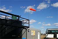 |
Critical to data quality during the second monitoring survey at the CO2 injection site in Russell County, Kansas, has been the avoidance of excessive wind noise. March is a month known to be particularly windy through central and western Kansas. Noise from wind is difficult to attenuate using post-acquisition processing techniques on seismic data due to its somewhat random arrival pattern and broadband spectral characteristics. Major efforts were taken to minimize the recording of excessive wind noise. Most significant of these efforts were recording at night and only recording when winds were less than 15 mph (an empirically based wind speed based on noise levels observed at the seismograph during recording). As a result of these strict acquisition guidelines, several days might pass without data being recorded while other days more than 240 shotpoints were recorded in a twenty-hour work period.
| Click on any image to view a larger version | ||
|---|---|---|
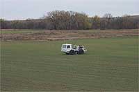
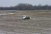
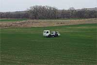
| Figure 2--Seasonal changes Nov. 2003 (left), Jan. 2004 (middle), to March 2004 (right). | ||
 |
 |
 |
Shot gathers from the three surveys completed so far are, in general, of very good quality (Figure 3). Repeatability of reflection amplitudes and source-wavelet characteristics is better than expected and clearly demonstrates the advantages of consistency in all aspects of the data acquisition on time lapse. This repeatability has greatly reduced the importance of computational-equalization techniques that have been essential to time-lapse analysis on most other 4-D seismic surveys. Coherent energy arrivals with hyperbolic moveout, characteristic of reflections, are interpretable throughout the primary depth interval. More than a dozen individual reflections returning from between the Stone Corral Anhydrite and Arbuckle are easily identifiable on the shot gathers with guidance from the downhole survey acquired in #16, the synthetic seismogram, and published data from this general area.
| Click on any image to view a larger version |
|---|
| Figure 3--Comparison of shot gathers from three trips. Before CO2 injection (top), after 6 weeks of CO2 injection (middle, ~200,000 gallons), and then after a little more than three months of CO2 injection (bottom, ~450,000 gallons). Reflections from the Lansing-Kansas City (L-KC) should be arriving between 550 and 590 msec, depending on source offset. Exact time depths are determined from VSP and synthetic seismograms produced from nearby sonic logs. The boxed area is enlarged in Figure 4. |
 |
 |
 |
Meaningful correlation of the synthetic traces with traces from a shot gather requires estimates of reflection-arrival time based on source-to-receiver offset, time shifts that are compensated for on vertical incidence, and CMP-stacked sections using the NMO correction. Based on reflection-curve modeling, reflections from the L-KC should arrive at times ranging from 548 msec for vertical-incident traces to 610 msec for offsets of 900 m. Using this general relationship, the exact set of reflection wavelets returning from the injected interval can be identified on shot gathers
| Click on any image to view a larger version |
|---|
| Figure 4--Time slice from the depth range of interest; baseline survey (top), first monitor survey (Jan. 2004) (middle), and second monitor survey (March 2004) (bottom). Clearly with the passing of time and increased volume of CO2-the reflection evident within the box at approximately the correct time for the L-KC-appears to possess steadily increasing amplitude. This increased amplitude could be indicative of increased reflectivity resulting from changes in layer characteristics. |
 |
| Figure 5--Magnified comparison of reflections within the time depth approximately correct for the L-KC interval. Blue and yellow highlights correlate to same zones in Figures 3 and 4. |
 |
 |
Using the time-to-depth conversion extracted from the downhole survey conducted in #16 (Figure 6), it is possible to bulk time-correct the synthetic seismogram (Figure 7) for the normal inaccuracy in absolute time resulting from estimating overburden velocity. As usual, these errors range from less than a percent in areas with an abundance of ground truth to as much as 10 percent when no other information but the sonic log is available to help estimate replacement velocities. Using local well data only, the L-KC interval was estimated to be at a time depth of around 535 msec. Incorporating the VSP and manual wavelet-correlation techniques, the actual arrival time of the top of the L-KC on seismic data is around 548 msec. Using the VSP for the first-arrival information alone more than justifies the expense of getting these borehole data. Correlations between borehole and surface seismic are critical to accurately defining the wavelet returning from the L-KC. Considering the producing interval, and therefore the interval the CO2 is being injected into, is only 15 ft thick and equates to just a little more than 1 msec, it is imperative to identify the L-KC reflection within a few tenths of a percent.
| Figure 6--Uphole/VSP survey conducted in Colliver #16. Black arrow indicates first arrival of seismic energy from source at hydrophone 2270 ft below ground. |
 |
| Reverse energy is tube wave bouncing off weight hanging from bottom of cable carrying hydrophones. |
 |
| Click on image to view a larger version |
|---|
| Figure 7--Synthetic seismogram generated by extracting source wavelet from cross-correlation of synthetic and ground force. L-KC interval is clearly indicated by complex doublet waveform. Once time-corrected the L-KC reflection will begin at around 548 msec. |
 |
A 3-D seismic volume produced for the baseline survey provides an excellent look at preliminary data quality (Figure 8). At this very early stage of the data processing, reflection events look quite good and only lack some of the sitewide coherency generally associated with seismic data from this depth interval and in this part of Kansas. However, considering the excellent data quality evident on shot gathers and with improved velocity analysis and statics, these data will provide the necessary quality to test the effectiveness of low-cost, minimal-deployment 3-D to monitor CO2 injection from both the enhanced oil recovery and sequestration perspectives.
| Click on image to view a larger version |
|---|
| Figure 8--3-D display with cross-line and in-line sections and a time slice at 560 msec. |
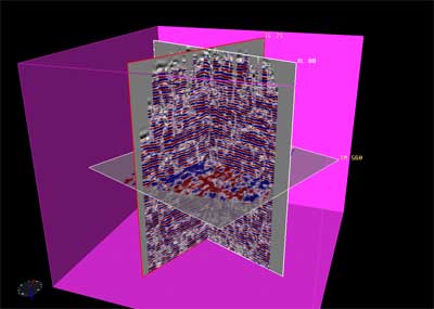 |
A time slice taken at 560 msec possesses subtle variations in reflection amplitude around this site (Figure 8). These changes in amplitude are likely indicative of changes in properties within the interval imaged. Considering the 'C' zone is just a little more than 1 msec thick, it will be imperative to have an accurate velocity model prior to detailed analysis of subtle amplitude variations.
|
Kansas Geological Survey, 4-D Seismic Monitoring of CO2 Injection Project Placed online June 9, 2004 Comments to webadmin@kgs.ku.edu The URL is HTTP://www.kgs.ku.edu/Geophysics/4Dseismic/Reports/Jun9_2004/index.html |