|
|
|
|
Jan. 2004 Site Visit--First Monitoring Survey |
|
|
|||
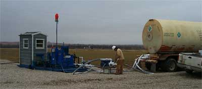
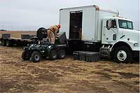
Deployment of recording equipment for the first 3-D monitoring survey began on January 17, 2004, approximately 6 weeks after the baseline 3-D survey and start of CO2 injection at the 10 acre enhanced oil recovery (EOR) demonstration site in southeastern Russell County, Kansas (Figure 1). Based on rough reservoir model estimations and the assumption CO2 is moving uniformly away (in the horizontal direction) from the injection well, the CO2 front should be at least 75 m, roughly 7 bins or subsurface seismic sample points, out from the injection well.
| Click on any photo to view a larger version |
|---|
| Figure 1--Kevin Axelson, Foreman for Murfin Drilling Company, monitors CO2 pressure. |
 |
In November 2003, just prior to initiation of the CO2 injection, a 3-D baseline survey of over 800 shot stations was conducted (Figure 2). High-resolution GPS was used to navigate the site and insured each source location would be reoccupied within 0.5 m on all subsequent acquisition trips. Besides navigation the DGPS system was programmed to provide a digital terrain map with an overall accuracy of better than 0.5 cm for each occupation point (Figure 3). Baseline reflection data were acquired intermittently over five days with stoppages for excessive wind, construction around the tank battery, and activity associated with well rework rigs. Night recording proved beneficial in minimizing wind and cultural noise.
| Click on any photo to view a larger version | |
|---|---|
| Figure 2--Vibrator tracking log showing all source stations occupied and routes driven. |
Figure 3--Digital terrain map from vibrator. |
 |
 |
Data quality from the baseline survey was excellent (Figure 4). Data were cross-correlated with the synthetic pilot trace after whole trace gain was applied, boosting the amplitude of the high frequency signal (1 second AGC scale). After correlation, coherent noise with an arrival pattern that changed from sweep-to-sweep (vehicles) was removed by zeroing affected portions of the data. Once the signal-to-noise ratio was maximized on each correlated sweep the last four sweeps (five sweeps were recorded at each site, but the first sweep was only used to seat the base plate) were then vertically stacked.
| Click on any photo to view a larger version |
|---|
| Figure 4--Correlated shot gather from station 19047, near center of receiver spread. |
 |
With simple spectral balancing (band-limited spiking deconvolution) the dominant frequency of the reflection increased from around 70 Hz to over 100 Hz, which equates to an improvement in resolution potential from 35 ft to around 25 ft at depths in excess of 3000 ft (600 msec) (Figure 5). As the data processing continues, the dominant frequency from 3000 ft could exceed 150 Hz, thereby providing vertical resolution potential of around 15 ft with an upper usable corner frequency of over 200 Hz, making the thinnest possible bed resolution at around 12 ft within the Lansing-Kansas City (L-KC) formation. Approximate two-way travel time of the interval of interest (L-KC) using NMO calculated average velocities is 600 ms. Several high quality reflections are evident between 500 and 800 msec. The top of the Arbuckle is likely the reflection at around 750 msec at longer offset traces with basement around 800 msec (Figure 5). Processing of the 3-D baseline data set into a stacked volume has commenced and should be completed by mid-February 2004.
| Click on any photo to view a larger version |
|---|
| Figure 5--Four shot vertical stack with spectral balancing. |
 |
Without doubt equipment upgrades and prototype components used to acquire these 3-D data more than doubled the overall signal-to-noise ratio and noticeably boosted the dominant frequency (Figure 6). Walkaway test acquired during August of 2002 using a 240-channel Geometrics Strataview seismograph (21 bit A/D) and IVI minivib I (1500 ft-lbs @ 200 Hz) with the standard factory valve produced data with excellent potential and quite adequate for the proposed 4-D monitoring project (Figure 6). However, upgrading the seismograph from 21 to 24 bits of dynamic range (going from a Geometrics StrataView to a distributed Geometrics Geode system) and quadrupling the power output of the vibrator by going to a minivib II w/high output Atlas rotary valve dramatically elevated the potential effectiveness of this technique to monitor, track, and allow prediction of CO2 movement with little increase in overall cost.
| Click on any photo to view a larger version |
|---|
| Figure 6--2-D shot gather acquired during August 2002 testing w/mini I and Strataviews. |
 |
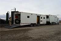
Equipment was transported to the field site in two semi-trailers (Figure 7). One hauled cables, phones, and vibrator (Figure 7a), while the other transported the ATVs used to haul cables and phones and house the recording equipment (Figure 7b). The semi-tractor used to move the ATVs and seismograph to the site also houses the mobile processing facility (MPC), which contains three workstations, two printers/plotters, and enough desk space for three processors (Figure 7b). All on-board computers are connected to each other and the seismograph via Ethernet.
| Click on any photo to view a larger version | |
|---|---|
| Figure 7 (a)--transports cables, phones, and vibrator. | Figure 7 (b)--transports ATVs and seismograph. |
 |
 |
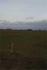
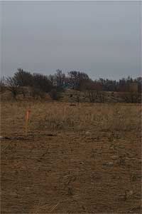
Time-lapse analysis of these two data sets (baseline and this the first of 11 3-D monitoring surveys) should require minimal if any special equalization procedures to compensate for changes in ground or recording conditions. Data acquisition on this first monitoring survey will mimic the baseline survey as closely as possible. Ground conditions across the site are nearly identical to what they were 2 months ago (Figure 8). With no appreciable new moisture and with ground conditions that were already extremely dry, from a seismic data perspective surface or near-surface conditions are unchanged between this survey and the baseline 3-D survey collected 6 weeks ago.
| Click on any photo to view a larger version | |
|---|---|
| Figure 8--Ground condition on January 17. Air temperature was 40° F and wind at 25 mph. | |
 |
 |
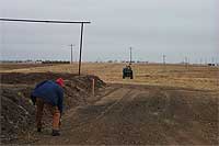
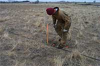
Cables were laid along receiver stakes placed during baseline survey (Figure 9a). Geophones were planted in the same locations (+/-10 cm) and with nearly identical coupling (Figure 9b). To insure as near identical recording conditions as possible no data will be recorded when wind speeds are in excess of 15 mph, with reluctance to record when the wind exceeds 10 mph. These general ground rules for recording in this notoriously windy area were used during the recording of the baseline survey and will be used for all 3-D monitoring surveys.
| Click on any photo to view a larger version | |
|---|---|
| Figure 9 (a)--cable laid w/ATV along stakes. | Figure 9 (b)--geophones planted at surveyed stakes. |
 |
 |
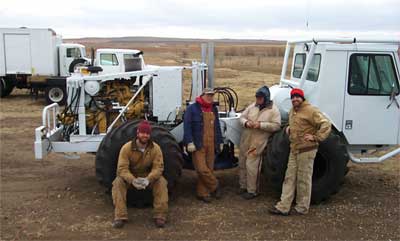
A hearty collection of students and staff laid the cables and phones on this blustery day in January (Figure 10). Key to time-lapse monitoring is consistent geophone plants, source coupling, and meticulous attention to detail, insuring a fully repeatable survey.
| Click on any photo to view a larger version |
|---|
| Figure 10--Left to right--Neb Cabrilo, David Thiel, David Laflen, and Brett Engard. |
 |
|
Kansas Geological Survey, 4-D Seismic Monitoring of CO2 Injection Project Placed online Jan. 21, 2004 Comments to webadmin@kgs.ku.edu The URL is HTTP://www.kgs.ku.edu/Geophysics/4Dseismic/Reports/Jan20_2004/index.html |