![]()
Prev Page--Ground Water || Next Page--Water Quality
Hydrologic Properties of Water-Bearing Materials
The quantity of ground water that an aquifer will yield to wells depends upon the hydrologic properties of the material forming the aquifer. The hydrologic properties of greatest significance are its ability to transmit and to store water, as measured by its coefficients of transmissibility and storage. Controlled aquifer tests in the field provide the data required to compute these coefficients.
The coefficient of transmissibility (T) may be defined as the rate of flow of water, in gallons per day, through a vertical strip 1 foot wide and extending the full height of the saturated thickness of the aquifer, under a hydraulic gradient of 1 foot per foot, at the prevailing temperature.
The coefficient of storage (S) may be defined as the change in the stored volume of water per unit surface area of the aquifer per unit change in the component of head normal to that surface.
The field coefficient of permeability (P) can be computed bv dividing the coefficient of transmissibility by the aquifer thickness (m). The field coefficient of permeability of an aquifer may be defined as the rate of flow of water, in gallons per day, through a square foot of its cross section, under a hydraulic gradient of 1 foot per foot, at the prevailing temperature.
Determinations of Transmissibility and Permeability
Aquifer tests were made using two wells deriving water from the Ogallala Formation to determine the coefficients of transmissibility and permeability of the Ogallala in Wallace County. Values of transmissibility were computed from the test data by the methods generally referred to as the Thiem method, the Theis nonequilibrium method, and the Jacob modified nonequilibrium method.
Thiem Method
The Thiem method of determining the coefficients of transmissibility and storage of water-bearing material is based on the rate of discharge of a pumped well and the drawdown in two or more observation wells at different known distances from the pumped well. The Thiem equation (Wenzel, 1942, p. 81), expressed in terms of transmissibility instead of permeability, is
in which T is the coefficient of transmissibility, in gallons per day per foot
Q is the rate of discharge of the pumped well, in gallons per minute
r1 and r2 are distances of two observation wells from the pumped well, in any unit
s1 and s2 are drawdowns of water level at distances r1 and r2, in feet
To apply the Thiem equation some convenient elapsed pumping time, t, is selected after the water levels in the observation wells reach a steady rate of decline. When the values of drawdowns, s, are plotted on the arithmetic scale of semilogarithmic paper and the values of distances, r, are plotted on the logarithmic scale, the data should form a straight line. From this line the change in drawdown per log cycle, Δs, is determined, and the Thiem equation is reduced to
Using this same line and extrapolating it to the zero-drawdown axis, the storage coefficient may be calculated by the following equation:
where S is the coefficient of storage
T is as previously defined
t is the time since pumping started, in days
r0 is the distance intercept on the zero-drawdown axis, in feet
The Thiem method of determining the coefficient of transmissibility is based on the theory that the aquifer is homogeneous throughout, but because aquifers are not perfectly homogeneous a probable error in the value of T is introduced. Some aquifers are so heterogeneous that the drawdown rate in aquifer tests is slowed in one or more of the observation wells and perhaps accelerated in others, thus giving a false slope to the line used in determining a value for Δs.
Theis Nonequilibrium Method
The Theis nonequilibrium method of determining the coefficients of transmissibility and storage is based on the rate of discharge of a pumped well and the rate of change of drawdown in one or more observation wells. The Theis nonequilibrium equation is
s is the drawdown in an observation well, in feet
r is the distance from pumped well to observation well, in feet
Q is the rate of discharge of the pumped well, in gallons per minute
T is the coefficient of transmissibility, in gallons per day per foot
S is the coefficient of storage expressed as a decimal fraction
t is the time since pumping began, in days
The integral expression is written symbolically as W(u) and is read as the "well function of u." The integral expression cannot be integrated directly, but its value is given by the series
Two unknowns and the nature of the integral expression make an exact analytical solution impossible, but Theis devised a graphical method of superposition that makes it possible to obtain a simple solution of the complex equation.
In this method a type curve is plotted on logarithmic paper with W(u) plotted along the vertical axis and 1/u along the horizontal axis to form a type curve (Wenzel, 1942, p. 88-89). If values of s obtained in one observation well are plotted against values of t on logarithmic paper of the same scale as the type curve, the curve of the observed data will conform to a part of the type curve. The data curve is superposed on the type curve, the axes of the two curves being held parallel and in a position that best fits the data curve to the type curve. The selection of a match point common to both curves provides the data needed to solve the Theis equation, which in simple form reduces to
For convenience a match point may be selected at the intersection of one of the major axes of the type curve, for example where 1/u = 10, or where 1/u = 100.
Jacob Modified Nonequilibrium Method
From the Theis equation, Cooper and Jacob (1946) developed the following formula:
where Q and T are as previously defined
t1 and t2 are two selected times since pumping started in any convenient units
s1 and s2 are the respective drawdowns, in feet, at the noted times
If the observed drawdowns for each well are plotted on the arithmetic scale and the values of t are plotted on the logarithmic scale of semilog paper, the resulting plot should form a straight line if enough time has elapsed since pumping began. If t1 and t2 are chosen one log cycle apart, the Jacob modified nonequilibrium equation reduces to
where Δs is the drawdown per log cycle.
The coefficient of storage can be determined from the same semilog plot of the observed data by the following equation:
where S, T, and r are as previously defined, and t0 is the time intercept on the zero-drawdown axis, in days.
Aquifer Tests
Waugh Aquifer Test
An aquifer test was made in August 1960 using irrigation well 14-42-23dbb1, owned by E. M. Waugh. The well is 350 feet deep and yields water from the Ogallala Formation. A drillers log of the pumped well and a sample log of observation well 1W (14-42-23dbb2) are included with the logs of test holes and wells at the end of this report. Two observation wells were drilled at distances of 237 and 468 feet from the pumped well. The well was pumped at a rate of about 1,600 gpm, as measured frequently with a Hoff flow meter. Drawdown measurements in the pumped well and the two observation wells were made during the period of pumping and are given in Table 5.
Table 5--Drawdown of water level in pumped well and observation wells during the Ogallala aquifer test, August 1960.
| Time since pumping started, minutes |
Drawdown, feet | ||
|---|---|---|---|
| Pumped well |
Well 1W | Well 2W | |
| 1 | 0.07 | ||
| 4 | 0.46 | ||
| 7 | 0.96 | ||
| 8 | 0.30 | ||
| 9 | 1.25 | ||
| 11 | 1.46 | ||
| 13 | 1.64 | 0.60 | |
| 15 | 1.81 | ||
| 17 | 1.97 | ||
| 18 | 0.80 | ||
| 19 | 2.09 | ||
| 21 | 2.20 | ||
| 23 | 2.28 | ||
| 24 | 1.06 | ||
| 25 | 31.78 | 2.36 | |
| 27 | 2.44 | ||
| 28 | 1.20 | ||
| 30 | 32.42 | 2.49 | |
| 33 | 32.49 | ||
| 34 | 1.35 | ||
| 35 | 2.64 | ||
| 36 | 32.54 | ||
| 38 | 1.44 | ||
| 40 | 2.74 | ||
| 42 | 1.52 | ||
| 45 | 2.83 | ||
| 47 | 32.81 | 1.59 | |
| 50 | 2.92 | ||
| 52 | 1.62 | ||
| 53 | 33.00 | ||
| 55 | 3.01 | ||
| 57 | 1.75 | ||
| 60 | 33.10 | 3.08 | |
| 62 | 1.80 | ||
| 70 | 3.20 | ||
| 72 | 33.31 | 1.90 | |
| 80 | 33.44 | ||
| 85 | 33.34 | ||
| 87 | 2.02 | ||
| 90 | 33.52 | ||
| 100 | 3.44 | ||
| 102 | 2.10 | ||
| 106 | 33.64 | ||
| 120 | 33.79 | 3.54 | |
| 130 | 2.23 | ||
| 140 | 3.63 | ||
| 150 | 2.31 | ||
| 155 | 33.97 | ||
| 160 | 3.71 | ||
| 180 | 3.79 | 2.40 | |
| 182 | 34.08 | ||
| 210 | 34.15 | 3.87 | 2.49 |
| 240 | 34.22 | 3.92 | 2.55 |
| 270 | 3.98 | 2.60 | |
| 287 | 34.26 | ||
| 310 | 4.04 | ||
| 315 | 2.65 | ||
| 330 | 34.33 | ||
| 340 | 4.08 | ||
| 345 | 2.69 | ||
| 390 | 34.47 | ||
| 395 | 4.16 | ||
| 398 | 2.75 | ||
| 450 | 34.50 | ||
| 455 | 4.23 | ||
| 457 | 2.82 | ||
| 473 | 34.55 | ||
| 540 | 34.64 | ||
| 545 | 4.29 | ||
| 550 | 2.91 | ||
| 713 | 34.76 | ||
| 720 | 4.50 | ||
| 723 | 3.10 | ||
| 930 | 34.89 | ||
| 940 | 4.70 | ||
| 945 | 3.24 | ||
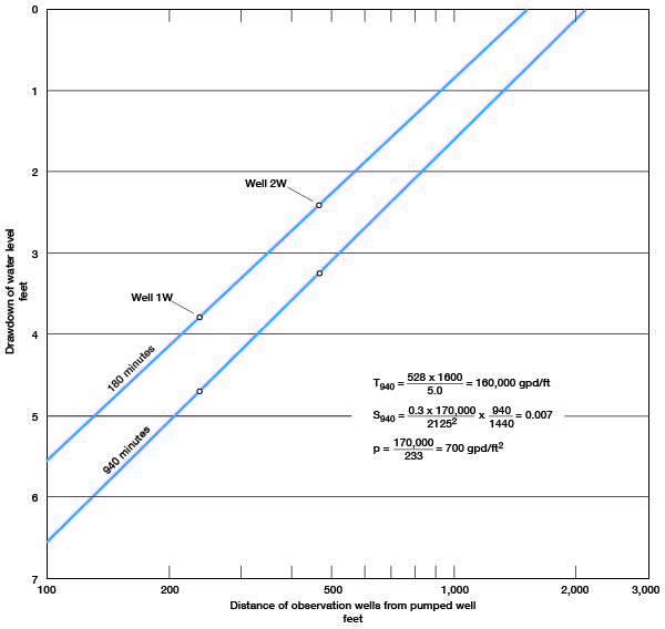
The coefficients of transmissibility shown in Figure 14 were determined by the Jacob modified nonequilibrium method. The coefficients computed from data from the pumped well and observation well 1W are believed to be correct; the larger coefficient of transmissibility obtained from data from observation well 2W is believed to be too high and can probably be accounted for by insufficient time for the drawdown to attain the correct slope because of the greater distance from the pumped well. The coefficients of transmissibility, permeability, and storage shown in Figure 15 were determined by the Thiem method.
Figure 14--Drawdown of water level measured in pumped well and observation wells during the Waugh aquifer test plotted against time since pumping started.
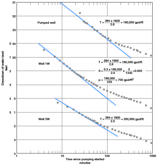
Figure 15--Drawdown of water level in observation wells at 180 and 940 minutes during the Waugh aquifer test plotted against distance from pumped well.
Holland aquifer test
An aquifer test was made in August 1960 using irrigation well 15-39-23cbc1 owned by G. W. Holland. The well is 234 feet deep and yields water from the Ogallala Formation. A drillers log of the pumped well and a sample log of observation well 1S (15-39-23cbc2) are included in Table 11. Two observation wells were drilled at distances of 120 and 237 feet from the pumped well. The well was pumped at a rate of about 1,300 gpm, as measured frequently by a Hoff flow meter. Drawdown measurements were made in the two observation wells during the period of pumping and are given in Table 6.
Table 6--Drawdown of water level in observation wells during the Holland aquifer test, August 1960.
| Time since pumping started, minutes |
Drawdown, feet | |
|---|---|---|
| Well 1S | Well 2S | |
| 3 | 2.52 | |
| 5 | 0.29 | |
| 7 | 3.34 | |
| 9 | 0.59 | |
| 11 | 3.63 | |
| 13 | 0.90 | |
| 15 | 3.80 | |
| 17 | 1.17 | |
| 19 | 3.98 | |
| 21 | 1.44 | |
| 23 | 3.99 | |
| 25 | 1.60 | |
| 27 | 4.05 | |
| 29 | 1.74 | |
| 31 | 4.09 | |
| 33 | 2.00 | |
| 35 | 4.15 | |
| 37 | 2.14 | |
| 39 | 4.18 | |
| 43 | 2.30 | |
| 45 | 4.21 | |
| 47 | 2.44 | |
| 50 | 4.26 | |
| 52 | 2.57 | |
| 55 | 4.29 | |
| 57 | 2.69 | |
| 60 | 4.31 | |
| 62 | 2.74 | |
| 68 | 4.34 | |
| 70 | 2.91 | |
| 75 | 4.37 | |
| 77 | 2.97 | |
| 84 | 4.40 | |
| 88 | 3.00 | |
| 96 | 4.45 | |
| 100 | 3.17 | |
| 112 | 4.49 | |
| 115 | 3.24 | |
| 134 | 4.54 | |
| 136 | 3.33 | |
| 150 | 4.58 | |
| 153 | 3.36 | |
| 173 | 4.62 | |
| 178 | 3.42 | |
| 212 | 4.60 | |
| 214 | 3.46 | |
| 242 | 4.66 | |
| 246 | 3.50 | |
| 300 | 4.72 | 3.54 |
| 390 | 4.69 | 3.58 |
| 505 | 4.66 | 3.60 |
| 815 | 4.91 | 3.71 |
| 855 | 4.92 | 3.73 |
| 1200 | 5.01 | 3.77 |
| 1620 | 5.15 | 3.89 |
| 2370 | 5.26 | 3.95 |
| 2975 | 5.39 | 4.05 |
| 3810 | 5.50 | 4.10 |
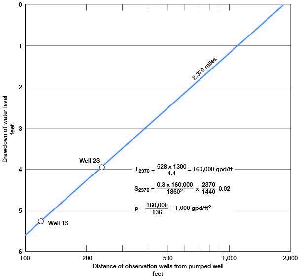
The drawdown of the water level in the observation wells is plotted against time on logarithmic paper in Figure 16. The Theis type curve was applied to determine the coefficient of transmissibility. The plot of the data deviates from the type curve for the later measurements and probably indicates that vertical drainage is occurring from the confining beds, in which case T is probably correct but S is not. The coefficient of transmissibility computed from data obtained from observation well 2S is believed to be correct. Observation well 1S seemingly did not respond to the drawdown as quickly as it should have and probably was partially plugged, at least during the early part of the aquifer test. The coefficients of transmissibility, permeability, and storage shown in Figure 17 were determined by the Thiem method.
Figure 16--Drawdown of water level in observation wells during the Holland aquifer test plotted against time since pumping started.
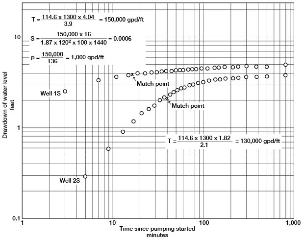
Figure 17--Drawdown of water level in observation wells at 2,370 minutes during the Holland aquifer test plotted against distance from pumped well.
Theoretical Predictions of Drawdowns
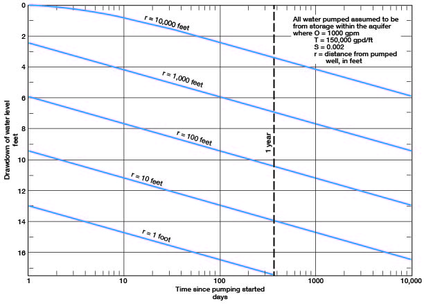
In order to predict future drawdowns the assumptions have been made that all water pumped came from storage within the aquifer, that pumping is continuous at a rate of 1,000 gpm, and that the water-bearing material has a T of 150,000 gpd per foot and an S of 0.002. The predictions of future drawdowns are in error to the extent that these assumptions are in error, but the predictions are probably of the right order of magnitude.
Figure 18 shows, under the assumed conditions specified specified, the drawdown of water level at any distance from a pumped well after 1, 10, 100, 1,000, and 10,000 days. After 100 days of pumping at a rate of 1,000 gpm, the drawdown at a distance of 1,000 feet will be about 6 feet. Figure 19 shows the rate of decline caused by pumping. A well pumped at 1,000 gpm for 10 days will cause about 4 feet of decline at a distance of 1,000 feet, and after 100 days about 6 feet of decline. The data indicate that the cone of influence will spread rapidly in response to pumping. Large-yield wells can interfere with each other unless the wells are spaced at considerable distances. When wells mutually interfere, the drawdown at any one point will be the sum of the drawdowns produced by each well.
Figure 18--Drawdown of water level at any distance from pumped well after pumping has begun.
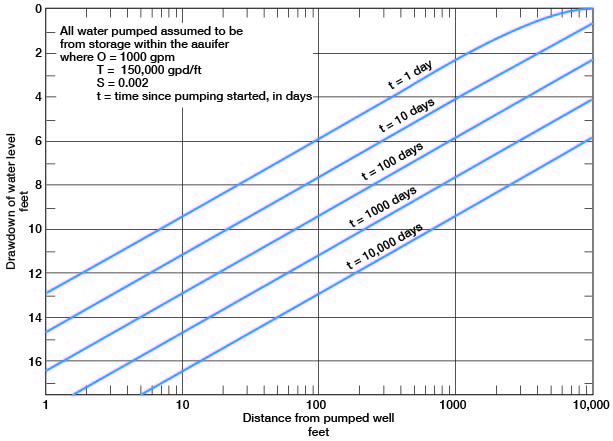
Figure 19--Drawdown of water level at any time after pumping has begun.
Movement of Ground Water
The quantity of ground water moving through a given cross-sectional area of water-bearing material can be calculated from the following formula:
Q = pAv = PIA
where Q = the quantity of water
p = the porosity of the material
A = the cross-sectional area
v = the velocity of the ground water
P = the coefficient of permeability, and
I = the hydraulic gradient.
The approximate rate of movement of water through the water-bearing materials can be calculated by applying the above formula transposed as follows:
v = PI/p
If P is expressed in gallons per day per square foot, I in feet per mile, and p in percent, then v, in feet per day, is given by the following formula:
v = PI/395p
The hydraulic gradient in the Ogallala Formation is approximately 12 feet per mile across the county. Aquifer tests indicate an average permeability of about 900 gpd per square foot. With an assumed porosity of 30 percent, the average velocity of the ground water is calculated to be
v = (900 x 12) / (395 x 30) = 0.9 foot per day, or
about 11 inches per day, or about 1 mile in 16 years.
Prev Page--Ground Water || Next Page--Water Quality
Kansas Geological Survey, Geology
Placed on web July 9, 2007; originally published November 1963.
Comments to webadmin@kgs.ku.edu
The URL for this page is http://www.kgs.ku.edu/General/Geology/Wallace/06_prop.html